Introduction to the Beta Distribution
If you are experimenting with Bayesian data analysis, the Beta Distribution will come up time and time again in the literature. The beta distribution is usually used to describe the prior distribution in Bayes equation. It can be very mathematically convenient to the Beta distribution as a prior, especially if the likelihood function is of the same function form (this is known as the conjugate prior).
The Beta distribution is a continuous probability distribution defined over the interval [0,1] and parameterized by two positive shape parameters a and b.
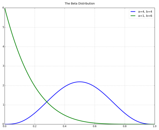
You can think of a and b in the prior as if they were previously observed data [1]. For example, if we were running a coin tossing experiment, you could think of a as the number of heads thrown, b as the number of tails thrown, and a + b as the total number of throws in the sample.
Now - lets look at the beta distribution over a wide range of a and b values.
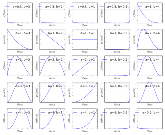
As you can see, a=1,b=1 is a uniform distribution. As you increase the value of a, the distribution shifts of the right, and as you increase the value of b, the distribution shifts to the left.
Binomal Data Analysis
The following explaination assumes:
- data is binomial: two possible outcomes (think heads or tails)
- observations are independent
- probability is stationary through time
- Bernoulli liklihood function
The goal of Bayesian analysis is to derive, either numerically or analytically the posterior probability distribution. To do this, you need to describe our ‘prior’ beliefs in a mathematical way. In other words, we need some formula that describes the prior probability on a scale of [0,1] and it needs to be a probability distribution (integral is 1). Event though you can technically use any probability distribution to describe your prior, when working with Bayes forumla, it convient if two of the following mathematical properties are satisfied
1) It is convient when the product of the liklihood function and the prior (numerator in Bayes rule) are of the same form as the prior. When this happens, the posterior will also be of the form of the prior. This quality allows us to include additional data and derive another posterior distribution of the same formula. Therefore, no matter how much data we include, we ALWAYS get a posterior of the same functional form [1]. (when this this happens, the prior is called the conjugate prior for the liklihood function [2])
2) We need the denomintor in Bayes Rule to be solved analytically. This depends on how the prior function relates to the liklihood function.
Given we are always seeking 1 and 2, and because our liklihood function is Bernoulli, our hopes and dreams are our prior is a conjugate prior and also is a Bernoulli distribution. If you look at it mathematically, given our likihood function is Bernoulli, you can see that if our Prior is also Beroulli, it will certainly make the product of the two easier to calculate:
Example:
N - number of heads
liklihood(N,p) = p^N*(1-p)^(1-N)
prior(Y,p) = p^A*(1-p)^A
liklihood(N,p) * prior(Y,p) = p^(N+A)*(1-p)^(1-N+B)
So because of reasons (1) and (2) above, we are seeking a prior with the same form as a Bernoulli distribution. The distribution is known as the Beta Distribution.
[1] “Doing Bayesian Data Analysis”, Chapter 5 [2] http://en.wikipedia.org/wiki/Conjugate_prior