The Law Of Large Numbers vs. The Central Limit Theorem
Two very important theorems in statistics are the Law of Large Numbers and the Central Limit Theorem.
The Law of Large Numbers
The Law of Large Numbers is very simple: as the number of identically distributed, randomly generated variables increases, their sample mean (average) approaches their theoretical mean.
The Law of Large Numbers can be simulated in Python pretty easily:
1
2
3
4
5
6
7
8
9
10
11
12
13
14
results = []
for num_throws in range(1,10000):
    throws = np.random.randint(low=1,high=7, size=num_throws)
    mean_of_throws = throws.mean()
    results.append(mean_of_throws)

df = pd.DataFrame({ 'throws' : results})

from IPython.core.pylabtools import figsize
from matplotlib import pyplot as plt
figsize(11, 9)
df.plot(title='Law of Large Numbers Explained Shown Graphically',color='r')
plt.xlabel("Number of throws in sample")
plt.ylabel("Average Of Sample")
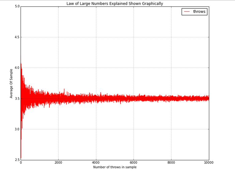
In this example, I am simulating throw a six-sided fair dice. The expected value is 3.5 and as you can see from the graph, when the same size is small, the mean is not close to 3.5, but as the sample size increases, the mean approaches 3.5.
The Central Limit Theorm
The Central Limit Theorem, in probability theory, a theorem that establishes the normal distribution as the distribution to which the mean (average) of almost any set of independent and randomly generated variables rapidly converges. The central limit theorem explains why the normal distribution arises so commonly and why it is generally an excellent approximation for the mean of a collection of data (often with as few as 10 variables).
1
2
3
4
5
6
7
8
9
10
11
12
13
14
15
16
17
18
19
20
21
22
23
24
25
26
27
28
29
30
31
32
33
34
35
36
samples_all = []
samples_all_exp = []
samples_all_possion = []
samples_all_geometric = []
mu = .9
lam = 1.0
size=1000

for number_in_sample in range(1,20000):
    samples = np.random.binomial(1, mu, size=size)
    samples_all.append(samples.mean())
    samples = np.random.exponential(scale=2.0,size=size)
    samples_all_exp.append(samples.mean())
    samples = np.random.geometric(p=.5, size=size)
    samples_all_geometric.append(samples.mean())
    samples = np.random.poisson (lam=lam, size=size)
    samples_all_possion.append(samples.mean())

df = pd.DataFrame({ 'binomial' : samples_all,
                     'poission' : samples_all_possion,
                     'geometric' : samples_all_geometric,
                    'exponential' : samples_all_exp})

from IPython.core.pylabtools import figsize
from matplotlib import pyplot as plt
figsize(11, 6)
fig, axes = plt.subplots(nrows=2, ncols=2)
df.binomial.hist(color='blue',ax=axes[0,0], alpha=0.9, bins=1000)
df.exponential.hist(ax=axes[0,1],color='r',bins=1000)
df.poission.hist(ax=axes[1,0],color='r',bins=1000)
df.geometric.hist(ax=axes[1,1],color='r',bins=1000)

axes[0,0].set_title('Binomial')
axes[0,1].set_title('Poisson')
axes[1,0].set_title('Geometric')
axes[1,1].set_title('Exponential')
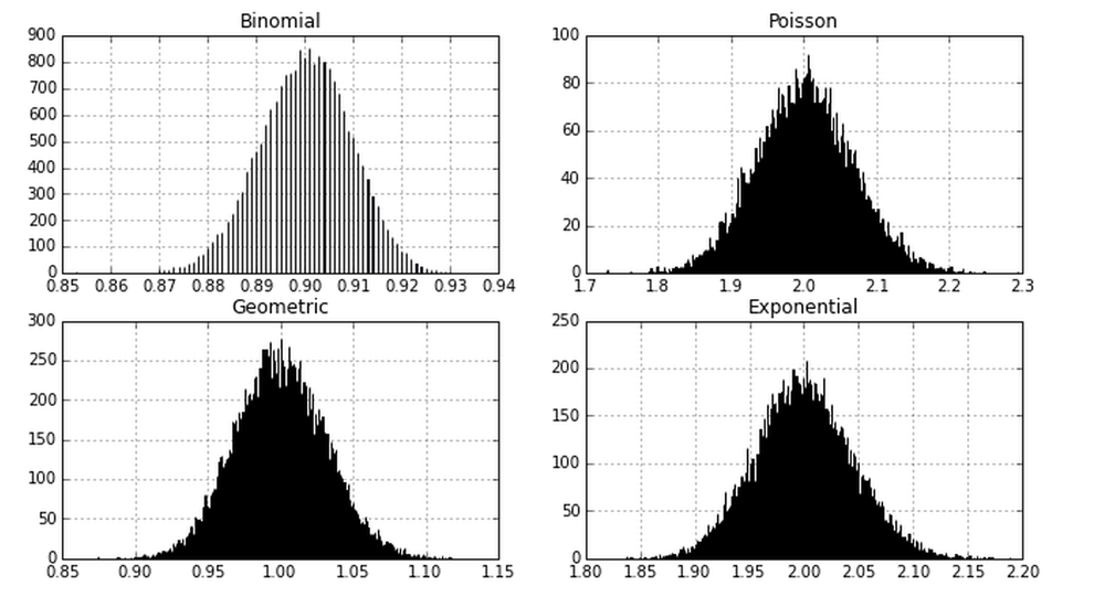
In the example above, I am creating random samples from four different probability distributions: Normal, Poission, Exponential, and Geometric. After the sample has been created, I take the mean of it and cache it. You can see that when I plot histograms of these means, they all follow the normal distribution, which is pretty amazing, because only 1/4 distributions is normal.